How Drone Altitude Control Relates to Dynamic Interest Rates in DeFi Credit Protocols
The world of Decentralized Finance (DeFi) provides new opportunities to optimize the financial mechanisms that relate to traditional finance. In the past, Ethereum’s design limitations confine the complexity of on-chain computation. However, with the recent innovations of higher performance smart contract blockchains like Solana, the door has been opened for faster and more efficient on-chain computation. We expect to continue to observe the optimization and refinement of many protocols as blockchains vertically scale.
Optimal control theory is a foundational concept in any engineering system. Whether you need to control the altitude of a drone with minimal overshoot or undershoot as quickly as possible, or continuously rebalance borrowing and lending rates in a DeFi credit protocol, optimal control theory is based around the idea the state of a system can be maintained by adjusting the input(s), assuming all the governing laws of the system have been formally defined.
PID Control Applied to Drone Altitude Control
Let’s consider a drone with four propellers (quadcopter) controlled by four DC motors, one for each propeller. The drone’s mission is to travel through an obstacle course in minimal time and at maximum speed. To avoid obstacles, the drone must be able to change its altitude quickly, but it must not overshoot or undershoot to avoid hitting objects above and below.
Let’s assume the drone is initially at 50 meters and needs to reach an altitude of 100 meters. The entire process needs to take less than 5 seconds, but the drone cannot overshoot or undershoot by more than 5% of the desired altitude (± 5 meters).
**Note: In a real-world scenario, there are constraints regarding the maximum voltage that can be applied to the DC motors, the maximum speed the DC motors can spin, etc.
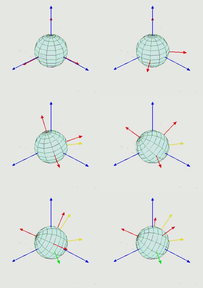
The location of the drone at a single point in time can be described by its height above the ground (z), its latitudinal and longitudinal coordinates (x and y respectively), and Euler’s angles, α, β, and γ, which describe the relative angles from each of the aforementioned axes.
Euler’s Angles:1
For simplicity of this example, let’s assume that voltage is supplied equally to all the motors and there is no change in Euler’s angles. Therefore, we can describe the movement of the drone in terms of z, z’ , and z’’.
We will adjust the speed of the motors to reach the desired altitude with the set of constraints. To accomplish this, we will use a proportional-integral-derivative (PID) controller. A PID controller constantly measures the difference in the desired state and the current state. The resulting error term is fed back into the input to influence that state. Intuitively, using the relationship between the speed of the motors and the drone’s altitude, we can increase the speed of the motors when the drone is below the desired altitude and decrease the speed of the motors when the drone is above the desired altitude.
The equation describing the state of the drone after ∆voltage is as follows:
altitude = previous altitude + (current voltage - previous voltage) * ωWhere the voltage is the control input and omega is the coefficient (usually less than 1) that accounts for the time it takes for the voltage signal to reach the DC motors. At t = 0, our previous voltage will be equal to the voltage required to supply the motors to make the drone hover.
We will now designate the control compensation u(t) that will be added onto the input at every time t as:
Where:
t is time
e(t) is the error term calculated at each t
τ is t minus 1
Kp is the proportional gain
Ki is the integral gain
Kd is the derivative gain
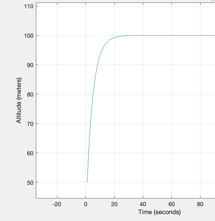
If we only focus on the proportional gain (Kp) and ignore Ki and Kd, the input compensation will never be greater than the error and we will never actually reach the desired altitude, we will only get infinitely close to the desired altitude. This is where the integral term and the derivative term come into play.
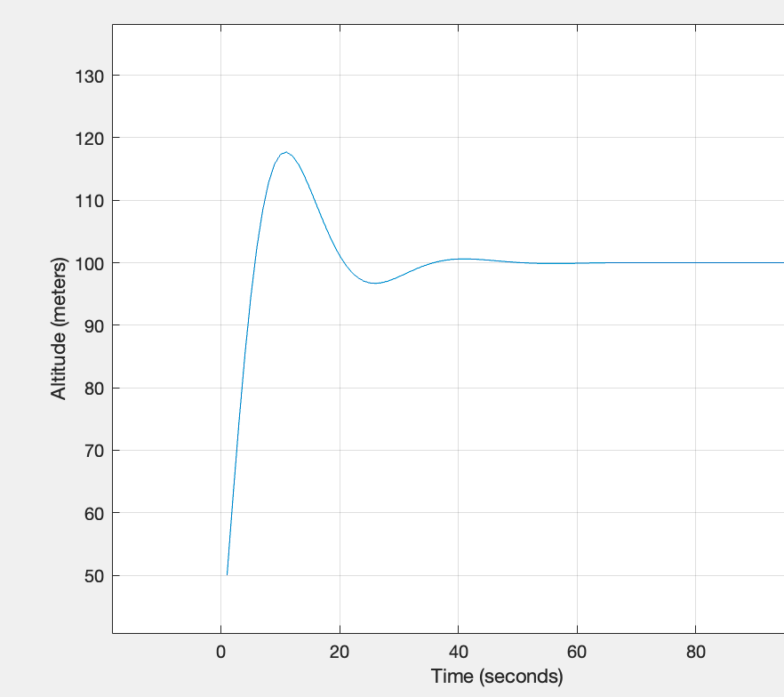
The integral gain (Ki) accounts for the area under the error vs time graph. This means that the larger the error is for a longer period of time, the greater integral term will create more aggressive compensation. To account for overshoot, this term will become negative as the current altitude exceeds the desired altitude. The addition of this term eliminates the error completely, reaching the exact desired altitude with no error.
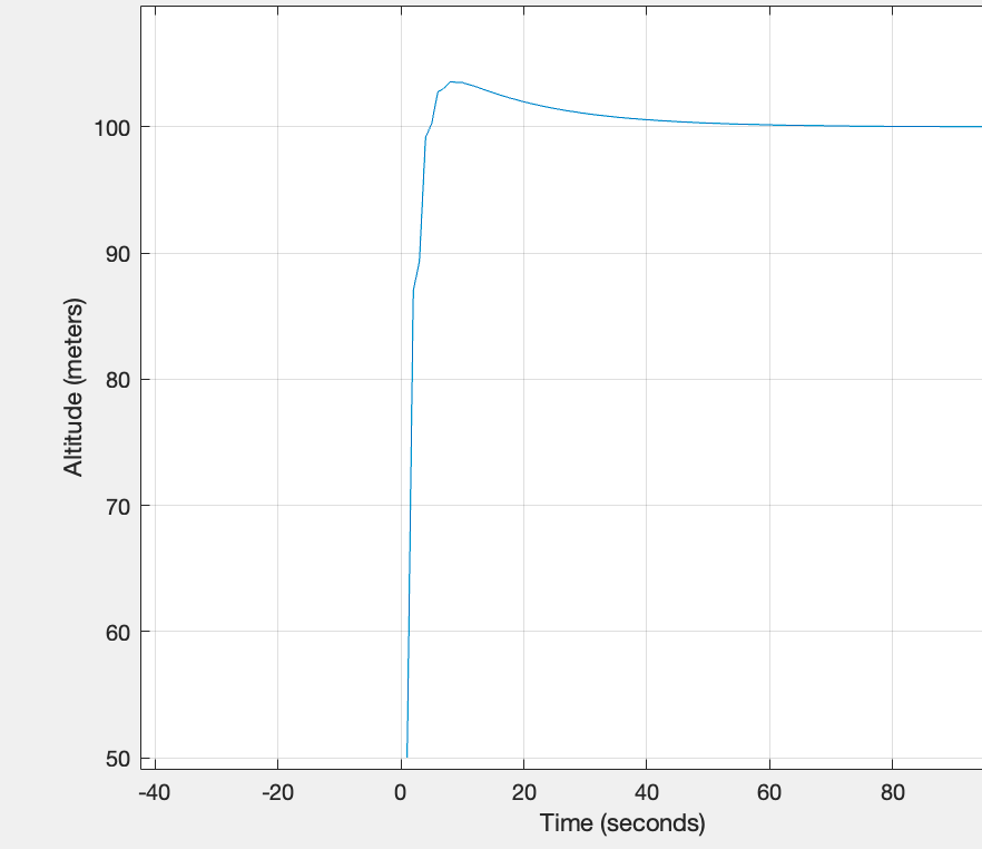
We now introduce the derivative gain (Kd), which minimizes the time required to reach the desired state. The derivative gain measures the rate of change (∆) of the current error - previous error, and will increase if ∆error is large and decrease when ∆error is small.
Here are the effects of altering Kp, Ki, and Kd:
Altitude vs Time with only Kp:
** On this graph it appears that the drone has indeed reached 100 meters, but this is because of the scale. As you zoom in, it in fact asymptotically approaches but never reaches 100 meters.
Altitude vs Time with Kp and Ki:
Altitude vs Time with Kp, Ki, and Kd:
These graphs illustrate how each of the gain values, Kp, Ki and Kd, will affect the state (altitude) of the drone. The next step is to “tune” the PID controller which is the process finding the optimal coefficients Kp, Ki, Kd. This process can be quite complex, but some methods include:
Ziegler-nichols Method (basic, but is reliable and produces consistently stable systems)
Online software in programs like MATLAB
Pole Placement in a Full State Feedback Loop (accurate, but difficult to iterate quickly due to pole behavior)
Linear Quadratic Regulator (LQR) (allows you to prioritize your constraints with a “cost function”)
The most commonly used method is the Ziegler-nichols approach due to its straightforward and formulaic approach. Depending on the constraints of the system, initially tuning the controller by hand can be a good exercise to visualize how certain gains can affect the system, whose behavior can vary drastically.
Even though the drone still overshoot the desired altitude in plot three, the drone reaches the 100 meter mark in a much shorter amount of time than in the first plot (which has no overshoot). At this stage, there is not a “right answer;” the solution set depends on pre-defined constraints/priorities of a system.
Now that we have developed a basic model describing the altitude of the drone, we could go much further to model the dynamics of the drone in more than the “z” direction. PID controllers could be constructed for other directions of motion, controlling the ground speed, turning radius, and generally any other aspect of the system by relating the motion to the input voltage.
After seeing the high-level design process that we used to construct and tune this controller for the drone, it becomes interesting when we apply it to DeFi. While the equations will not be the same, there are many parallels we can draw between the two fields to simplify our problem and better characterize the dynamics on a blockchain.
PID Control Applied to DeFi Credit Protocols
Today, DeFi credit protocols such as Aave and Jet use the linear-piecewise interest rate curve to describe the relationship between borrow/supply interest rates in order to maintain the optimal ratio of borrowed assets to supplied assets (called the optimal utilization ratio).2
Linear Piecewise Model (two piece)
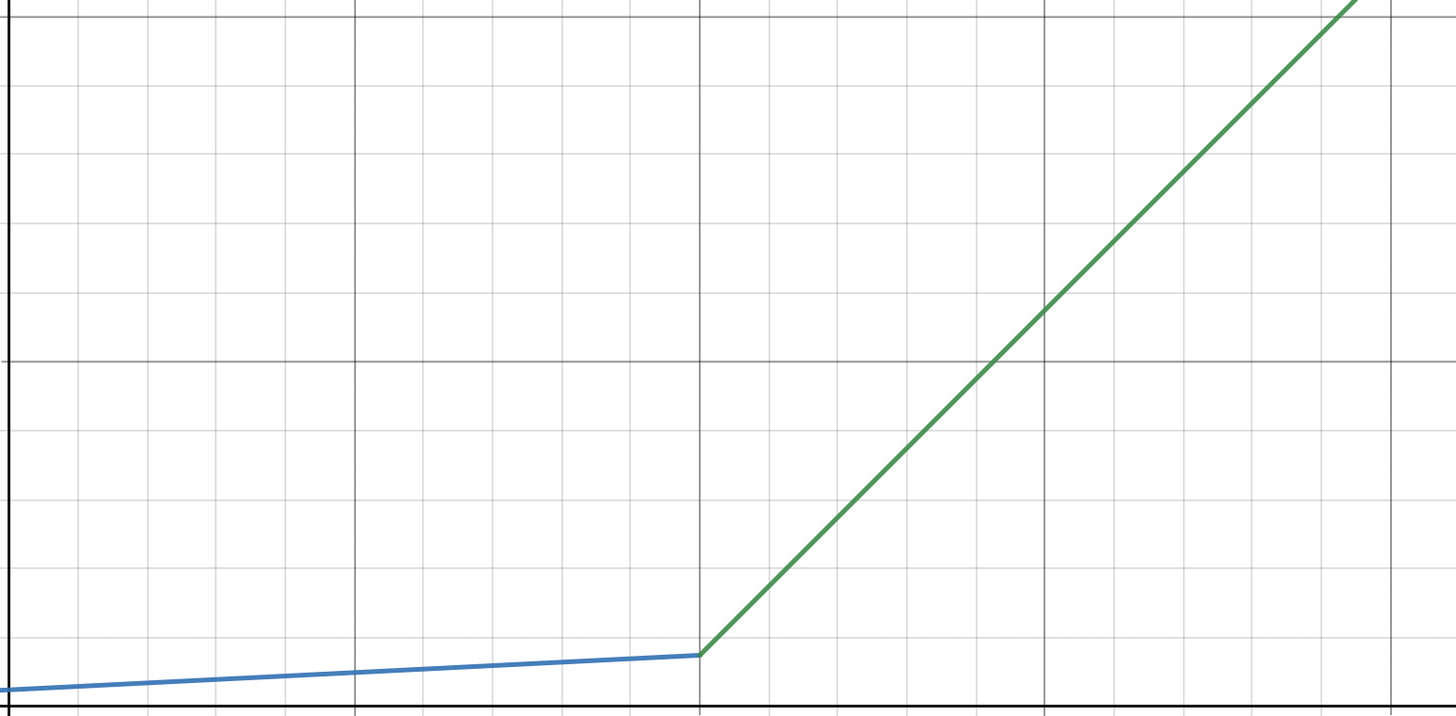
In the linear piecewise model used by Aave, borrow interest rates are calculated as a function of the utilization ratio. The moment when the slope of these lines change is defined on the x-axis as the optimal utilization ratio.
Linear Piecewise Model (three piece)
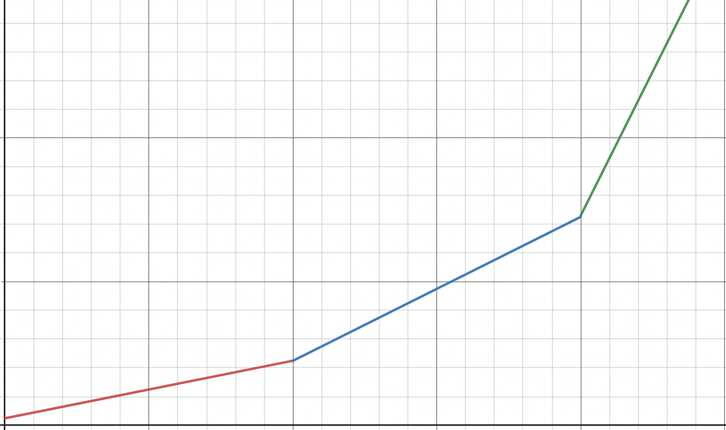
The three part piecewise function is an improvement on the two piece linear function used by Jet protocol. Instead of a single optimal utilization point, there are two optimal utilization points which is predicted to help increase capital efficiency.
When calculating the optimal utilization ratio, protocols must consider a tradeoff. If the ratio is high (close to 1), the assets in the pool are almost fully lended, approaching maximum capital efficiency while the pool runs the risk of becoming illiquid. Inversely, if the pool is not being lent out, the protocol is sacrificing capital efficiency for more security.
Now, we relate the problem back to the drone and its PID controller.
If we treat the optimal utilization ratio like the altitude and the borrow interest rate like the change in voltage, we arrive at this equation.3
utilization ratio = previous utilization ratio + (current borrow interest rate - previous borrow interest rate) * ωOmega is the delay at which the utilization ratio reflects the changes made in interest rates (similar to the time it takes for the voltage signal to reach the DC motors).
At t = 0, the previous interest rate is defined as the baseline interest rate across other DeFi protocols. Conceptually, this is similar to the voltage supplied to the DC motors to create a state of equilibrium, making the drone “hover.” The derivation of this baseline interest rate needs to be explored further, but will likely result from the development of a game-theoretic interest rate model that determines the “cost of money” depending on the supply/demand of a certain asset.
The constraints for this problem:
With an initial error of 40%, the current utilization ratio must equal the optimal utilization ratio within 5 seconds. The utilization ratio must maintain a ± 5% accuracy (of the optimal utilization) to ensure the pool never becomes over utilized.
In the models below, the baseline interest rate is arbitrarily chosen to be 5%.
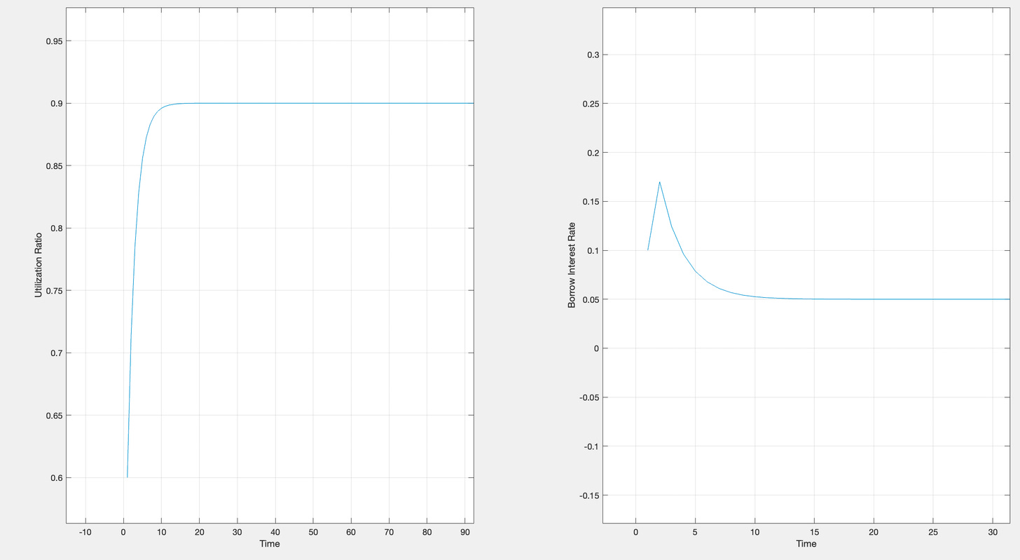
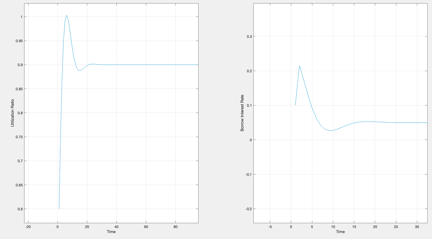
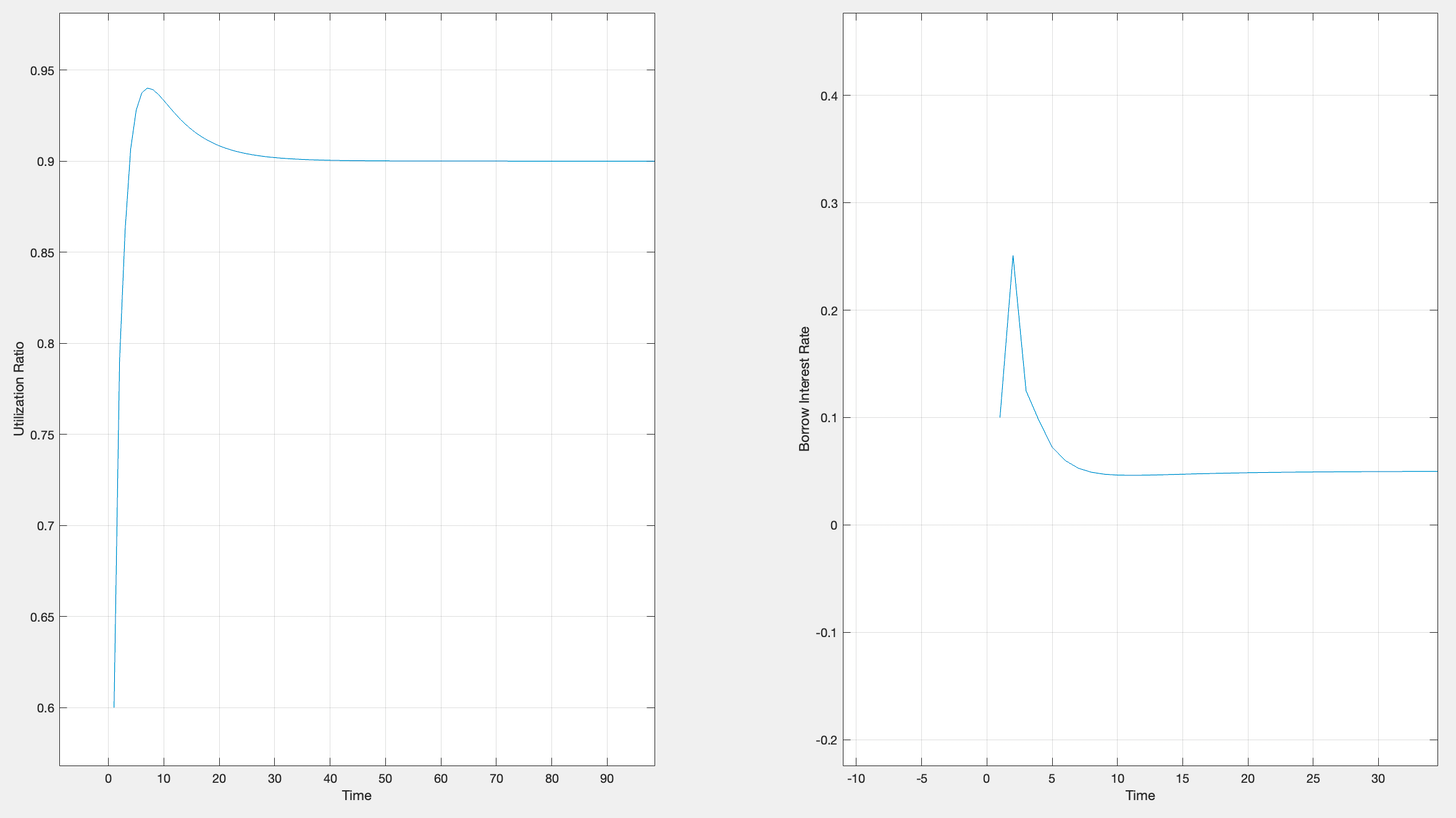
Here are the effects of using the same PID controller as the drone to control the state (utilization ratio) of a lending/borrowing pool when the initial utilization ratio is 60% and the optimal utilization ratio is 90%.
Utilization Ratio vs Time with only Kp:
Utilization Ratio vs Time with Kp and Ki:
Utilization Ratio vs Time with Kp, Ki, and Kd:
**Note: Observe that the interest rate peaks at the time where the change in utilization ratio is the greatest.
Additionally, the utilization ratio and borrow interest rate are both plotted with respect to time because the time represents the time after the last block that updated the current utilization ratio and before the next block that will update it again.
Even though there will likely be constraints that limit the ability to change interest rates so abruptly, implied by the last chart, our system is much more responsive than a linear one. Any change in utilization ratio that is outside a threshold will trigger trigger an increase or decrease in interest rates to achieve the optimal utilization ratio, minimizing the time during which a pool would be over/under-utilized.
Depending on the gain values of the PID controller, we can modify the responsiveness of the system, tailoring it to the constraints or limitations of a certain protocol.
There is plenty more work to be done on this problem and specifically:
Baseline interest rate calculations need to be explored
PID gain tuning techniques need to be implemented
Optimal utilization ratios are loosely defined and there needs to be a more systematic method of their calculation
In conclusion, this is an example of how a seemingly unrelated idea may be used to solve a problem in a completely different field. While this is a basic implementation of the PID controller, it is evident that there is strong correlation between the setup of a drone scenario when compared to a credit protocol. This manner of problem solving may push the envelope by enabling new processes and more efficient systems as they relate to DeFi.
Please subscribe to our newsletter here to receive more information!
By Patrick M
© 2022 cypher protocol
https://commons.wikimedia.org/wiki/File:Euler2a.gif
https://docs.aave.com/risk/liquidity-risk/borrow-interest-rate
https://docs.jetprotocol.io/jet-protocol/protocol/interest-rates-on-jet
https://members.delphidigital.io/reports/dynamic-interest-rate-model-based-on-control-theory/


